1 Overview
For our self-proposed final project for CSCI1470: Deep Learning, we implemented SqueezeNet with additional optimizations like Network Pruning, Quantization and Huffman Encoding. This allowed us to reduce SqueezeNet to ~0.80MB, which is x300 times smaller than AlexNet, easily fitting on edge devices like the ESP32 microcontroller.
2 Motivation
As deep learnings models rapidly grow in size - GPT-3 has 175 billion parameters - edge devices are often relegated to the role of data collection given their limited computing power and memory. However, we believe that edge devices have the potential for real-time data analysis and inference by running deep learning models locally. As such, we wanted to port image classification models to devices with extremely low computing power and memory like a microcontroller.
As SqueezeNet was originally an optimization of AlexNet and achieved the same accuracy with 50x fewer parameters, we wanted to see if we could further compress SqueezeNet by implementing additional optimizations.
3 Methodology
3.1 Preprocessing Data
Data is king when it comes to training deep learning models. The first order of things was to choose a suitable dataset. Though we initially intended to use the same dataset originally used by AlexNet, ImageNet, for a direct comparison, we ran into issues of availability of data and preprocessing difficulties. We then opted for the Intel Image Classification dataset which has 6 labels with around 25,000 images with a pre-formatted size of 150x150.

3.2 Just SqueezeNet
Our base implementation is just SqueezeNet on its own. Though SqueezeNet is often compared to AlexNet, their architectures are significantly different. AlexNet uses 5 convolutional neural networks (CNNs) followed by max-pooling layers and then fully connected layers. As shown below, SqueezeNet begins with a convolutional layer, then max pooling, then a series of FireLayers and max-pooling after, finished off with a convolutional layer, a global average pool, and a softmax layer for producing probabilities on the labels.
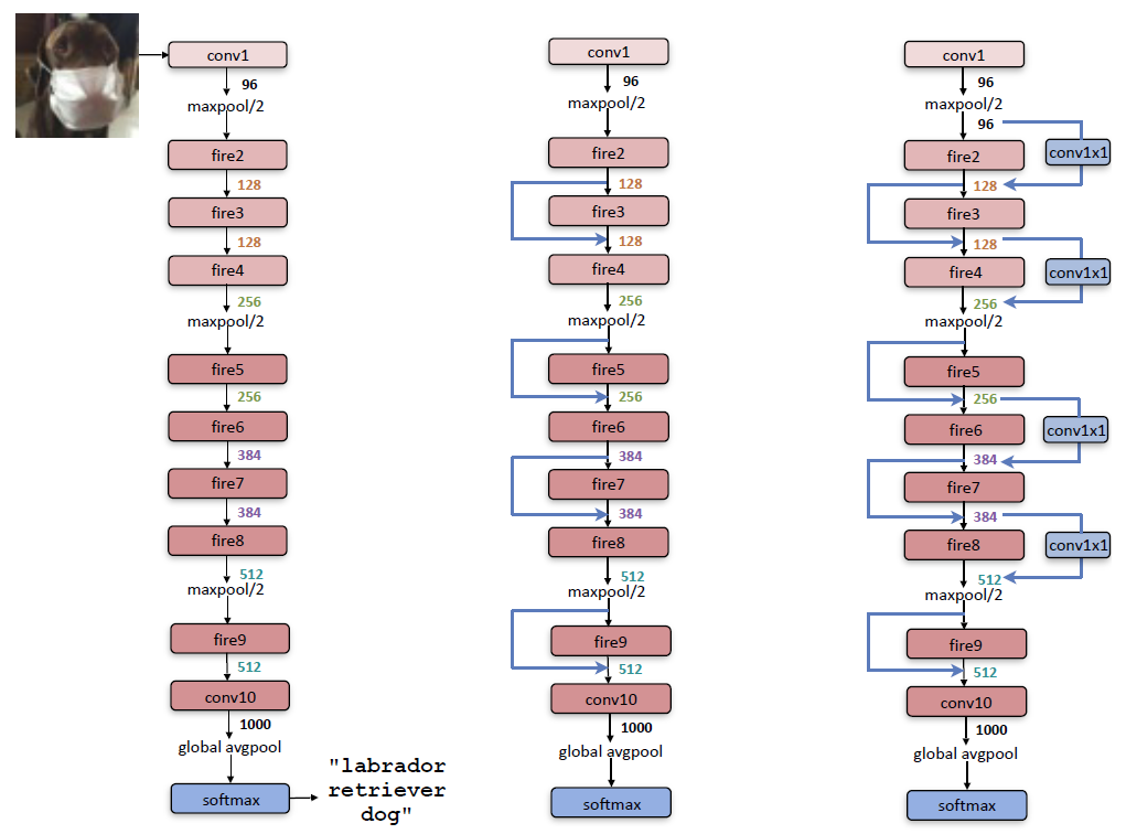
To reduce the model size, SqueezeNet uses 3 techniques: FireLayers, avoiding fully-connected layers and max-pooling.
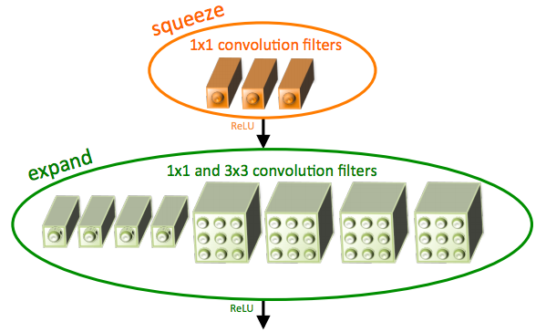
The FireLayers used throughout the network are composed of a “squeeze” layer (1x1 filters) and an “expand” layer that uses 1x1 and 3x3 filters. There are two benefits to this design: firstly, replacing the majority of 3x3 filters with 1x1 filters reduces the number of parameters by ~9 times. Secondly, by reducing the number of filters in the “squeeze” layer, this greatly reduces the number of connections between the “squeeze” layer and the “expand” layer, further reducing the total number of parameters. Check out our implementation of the FireLayer at /fire_mod.py.
As fully-connected layers hold an immense number of parameters (more than 85% of VGG’s 138 million parameters are in fully-connected layers), avoiding them is key to keeping the number of parameters small.
Several max-pooling layers are also used throughout the network in order to further reduce the number of parameters.
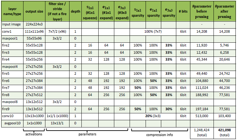
Note that because SqueezeNet was somehow unable to train well on the Intel Image Classification dataset, we opted to use SqueezeNet v1.1 with a slightly different architecture:
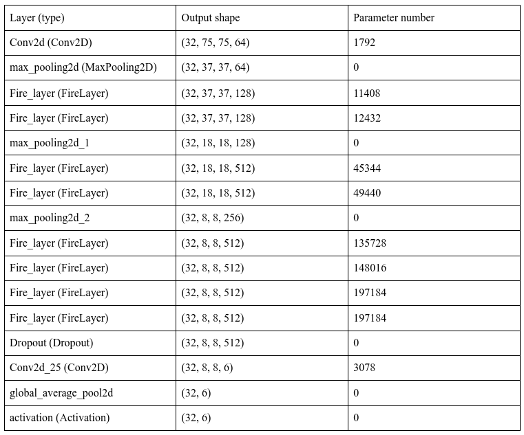
This baseline SqueezeNet implementation is only 3.71 MB, a x65 reduction in comparison to AlexNet’s 240 MB.
In the next few sections, I will discuss about the additional optimizations we implemented to further shrink SqueezeNet.
3.3 Optimization #1: Pruning
Pruning is a way of reducing the number of connections between layers. It is implemented in TensorFlow by gradually zeroing out the least impactful weights in the model to cut down on the number of useful weights.
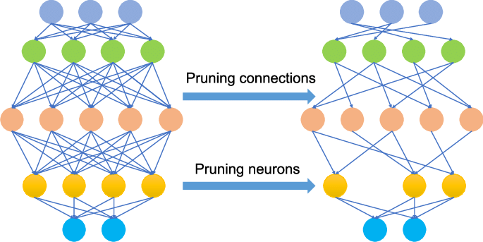
The benefits are two-fold: firstly, when we perform inference on these pruned models, the zeroed out weights can be skipped to improve model speed and efficiency without losing much accuracy since we’ve only removed the least impactful weights. Secondly, when the model is compressed (eg. using gzip), these zeroed out weights can be represented more compactly, further reducing the size of the model.
We use tfmot to implement pruning - tfmot.sparsity.keras.UpdatePruningStep() is a Keras callback that our model utilizes in each training stage in order to repeatedly prune our model. However, as tfmot was relatively new then, it did not support directly wrapping custom layers like our FireLayers for pruning. To work around this, we implemented our own functions wrap_layer_pruning() and strip_pruning_wrapping() to wrap and unwrap FireLayers for pruning.
Pruning further reduced SqueezeNet to 2.05 MB, a x117 reduction in comparison to AlexNet’s 240 MB.
3.4 Optimization #2: Quantization
Quantization involves converting the datatype of our weights from floats (32 bits) to ints (8 bits), reducing the number of bits required to represent each number and thus compressing the size of our model by approximately 4x.

Quantization is normally done post-training, but has the downside of significantly reducing our accuracy. To combat this, we use a quantization-aware model, which involves quantizing during training in addition to quantizing post-training. This ameliorates the issue of lower accuracy and even increases accuracy in certain cases. Check out quantization.py to see how we implement quantization.
Quantization further reduced SqueezeNet to 0.80 MB, a x300 reduction in comparison to AlexNet’s 240 MB.
3.5 Optimization #3: Huffman Encoding
Huffman coding is another compression technique that further reduces the number of bits required to represent each number, resulting in a 20% to 30% reduction in size.
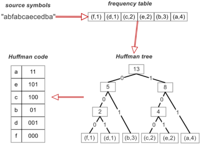
Huffman coding involves treating each unique number as a symbol and assigning each symbol a corresponding bit value. For example, we may represent the float 0.123456 as the bit 10. Higher frequency symbols are assigned smaller bit sizes and a codec containing each symbol to bit representation mapping is stored in this process. The final result is a weight tensor encoded into a sequence of bits along with a codec, which can be decoded and reshaped back into the original tensor at any point.
Although we were able to implement Huffman encoding using the dahuffman Python library, we were not able to fully integrate Huffman encoding into our pipeline due to the lack of support in Tensorflow modules. Check out our demo at huffman_opt.py that encodes a 500x500 32-bit tensor from ~8 MB to 0.56 MB.
4 Running on ESP32
By including a compressed model in a compiled demo project, and using the Tensorflow Lite Micro Interpreter, we were able to run SqueezeNet on the ESP32. The fact that this all fits within 2MB of application flash is impressive, and definitely not possible with the size of AlexNet!
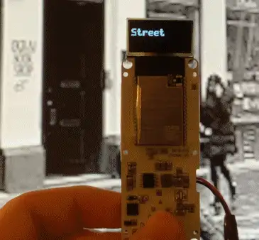
Check out our ESP32 demo at /ESP32_Demo_Classifier
5 Results
With pruning and quantization, we were able to reduce the size of SqueezeNet to a mere 0.80 MB!
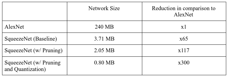
Despite being 300 times smaller than AlexNet, SqueezeNet w/ optimizations had a higher validation accuracy on the Intel Image Classification dataset compared to AlexNet:

6 Challenges
Although the base version of SqueezeNet was not particularly difficult to implement, challenges quickly arose when trying to accommodate our proposed compression techniques onto the model. This was mainly because the libraries we used (eg. tfmot) were fairly new and only worked in basic, restrictive contexts. This was further compounded by the relative sparseness of documentation online. As such, with custom FireLayers in our model, we often needed to dig into the source code of tfmot to devise hacks for working with our model.
For all our compression techniques, we were able to get a working version that demonstrated the utility of each technique, but were not always able to replicate the technique fully. This is because certain aspects, such as the prequantization training, are still actively being developed and are currently incompatible with our model.
Thanks Leonard, Eli and Stephen for working on this with me!